Feature Engineering in a Pipeline
Introduction
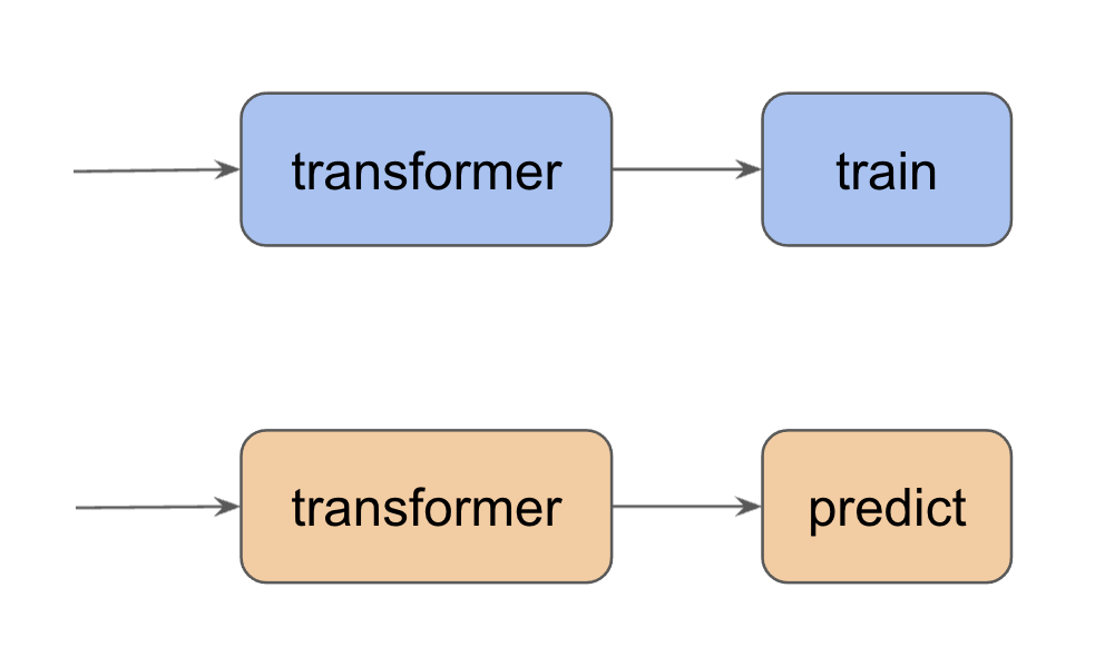
Feature engineering is a process of transforming the given dataset into a form which is easy for the machine learning model to interpret. If we have different transformation functions for training and prediction we may duplicate the same work and it’s harder to maintain (make some changes in one pipeline means we have to update the other pipeline as well).

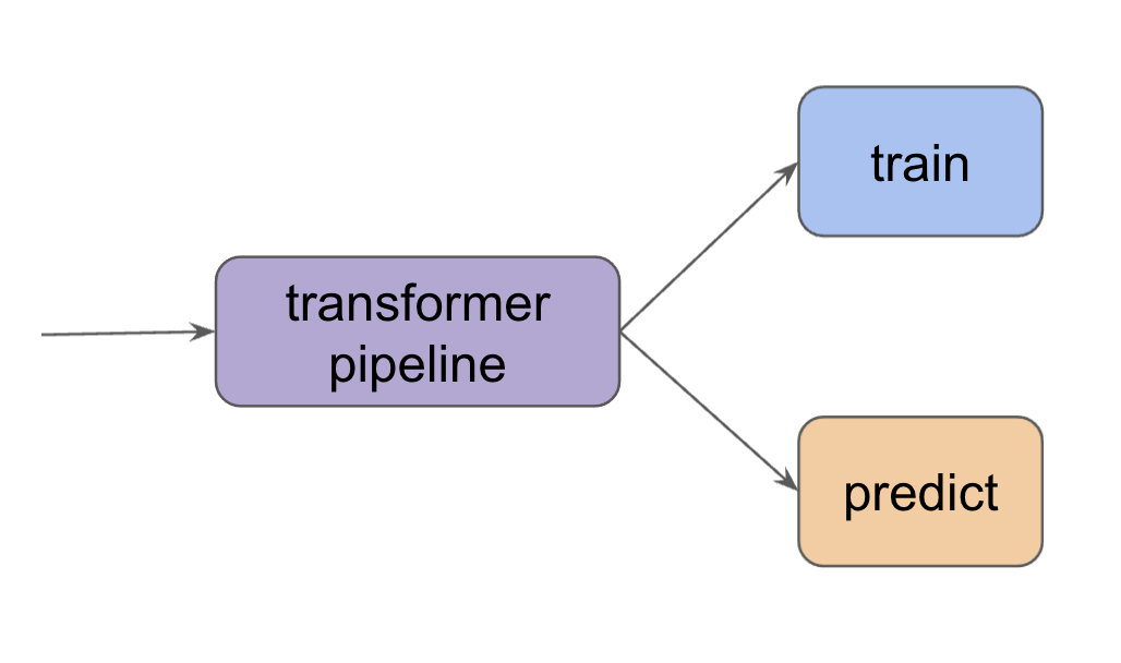
One common practice in producitionzing machine learning models is to write a transformation pipeline so that we can use the same data transformation code for both training and prediction.

In this article, we discuss how we can use scikit-learn to build a feature engineering pipeline. Let’s first have a look at a few common transformations for numeric features and categorical features.
Transforming Numerical Features
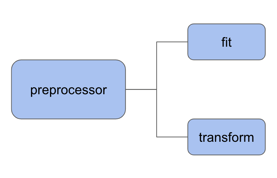
One thing I really like about scikit-learn is that I can use the same ‘‘fit’’ and ‘‘predict’’ pattern for data preprocessing. For a preprocessor, the two methods are called fit and transform.

We can use SimpleImputer to complete missing values and StandardScaler to standardize values by removing the mean and scaling to unit variance.
import pandas as pd
from sklearn.impute import SimpleImputer
from sklearn.preprocessing import StandardScaler
Let’s create a simple example.
data = {'n1': [20, 300, 400, None, 100],
      'n2': [0.1, None, 0.5, 0.6, None],
      'n3': [-20, -10, 0, -30, None],
    }

df = pd.DataFrame(data)
df
| n1 | n2 | n3 | |
|---|---|---|---|
| 0 | 20.0 | 0.1 | -20.0 |
| 1 | 300.0 | NaN | -10.0 |
| 2 | 400.0 | 0.5 | 0.0 |
| 3 | NaN | 0.6 | -30.0 |
| 4 | 100.0 | NaN | NaN |
We can have a look the mean of each column using the .mean() method.
df.mean()
n1    205.0
n2      0.4
n3    -15.0
dtype: float64
Here we create a SimpleImputer object with strategy="mean". This means we fill the missing value using the mean along each column.
num_imputer = SimpleImputer(strategy="mean")
We first fit our imputer num_imputer on our simple dataset.
num_imputer.fit(df)
SimpleImputer()
After fitting the model, the statistic, i.e., the fill value for each column, is stored within the imputer num_imputer.
num_imputer.statistics_
array([205. , 0.4, -15. ])
Now we can fill the missing values in our original dataset with the transform method. By the way, we can also apply fit and transform in one go with the fit_transform method.
imputed_features = num_imputer.transform(df)
imputed_features
array([[ 2.00e+01,  1.00e-01, -2.00e+01],
       [ 3.00e+02,  4.00e-01, -1.00e+01],
       [ 4.00e+02,  5.00e-01,  0.00e+00],
       [ 2.05e+02,  6.00e-01, -3.00e+01],
       [ 1.00e+02,  4.00e-01, -1.50e+01]])
type(imputed_features)
numpy.ndarray
The transformed features are stored as numpy.ndarray. We can convert it back to pandas.DataFrame with
imputed_df = pd.DataFrame(imputed_features,
    index=df.index, columns=df.columns)
imputed_df
| n1 | n2 | n3 | |
|---|---|---|---|
| 0 | 20.0 | 0.1 | -20.0 |
| 1 | 300.0 | 0.4 | -10.0 |
| 2 | 400.0 | 0.5 | 0.0 |
| 3 | 205.0 | 0.6 | -30.0 |
| 4 | 100.0 | 0.4 | -15.0 |
The cool thing is that now we can use the same statistic saved in num_imputer to transform other datasets. For example here we create a new dataset with only one row.
# New data

data_new = {'n1': [None],
      'n2': [0.1],
      'n3': [None],
    }

df_new = pd.DataFrame(data_new)
df_new
| n1 | n2 | n3 | |
|---|---|---|---|
| 0 | None | 0.1 | None |
We can apply num_imputer.transform on this new dataset to fill the missing values.
pd.DataFrame(num_imputer.transform(df_new),
    index=df_new.index, columns=df_new.columns)
| n1 | n2 | n3 | |
|---|---|---|---|
| 0 | 205.0 | 0.1 | -15.0 |
StandardScaler works in a similar way. Here we scale the dataset after the imputer step.
num_scaler = StandardScaler()
num_scaler.fit(imputed_df)
StandardScaler()
pd.DataFrame(num_scaler.transform(imputed_df),
    index=df.index, columns=df.columns)
| n1 | n2 | n3 | |
|---|---|---|---|
| 0 | -1.361620 | -1.792843e+00 | -0.5 |
| 1 | 0.699210 | -3.317426e-16 | 0.5 |
| 2 | 1.435221 | 5.976143e-01 | 1.5 |
| 3 | 0.000000 | 1.195229e+00 | -1.5 |
| 4 | -0.772811 | -3.317426e-16 | 0.0 |
Transforming Categorical Features
OneHotEncoder is commonly used to transform categorical features. Essentially, for each unique value in the original categorical column, a new column is created to represent this value. Each column is filled up with zeros (the value exists) and ones (the value doesn’t exist).
from sklearn.preprocessing import OneHotEncoder


cat_encoder = OneHotEncoder(handle_unknown='ignore')

data = {'c1': ['Male', 'Female', 'Male', 'Female', 'Female'],
      'c2': ['Apple', 'Orange', 'Apple', 'Banana', 'Pear'],
    }

df = pd.DataFrame(data)

df
| c1 | c2 | |
|---|---|---|
| 0 | Male | Apple |
| 1 | Female | Orange |
| 2 | Male | Apple |
| 3 | Female | Banana |
| 4 | Female | Pear |
Let’s first fit a one hot encoder to a dataset.
cat_encoder.fit(df)
OneHotEncoder(handle_unknown='ignore')
Note that the categories of each column is stored in attribute .categories_.
cat_encoder.categories_
[array(['Female', 'Male'], dtype=object),
 array(['Apple', 'Banana', 'Orange', 'Pear'], dtype=object)]
Here is the encoded dataset.
pd.DataFrame(cat_encoder.transform(df).toarray(),
    index=df.index, columns=cat_encoder.get_feature_names_out())
| c1_Female | c1_Male | c2_Apple | c2_Banana | c2_Orange | c2_Pear | |
|---|---|---|---|---|---|---|
| 0 | 0.0 | 1.0 | 1.0 | 0.0 | 0.0 | 0.0 |
| 1 | 1.0 | 0.0 | 0.0 | 0.0 | 1.0 | 0.0 |
| 2 | 0.0 | 1.0 | 1.0 | 0.0 | 0.0 | 0.0 |
| 3 | 1.0 | 0.0 | 0.0 | 1.0 | 0.0 | 0.0 |
| 4 | 1.0 | 0.0 | 0.0 | 0.0 | 0.0 | 1.0 |
We can now use cat_encoder to transform new dataset.
data_new = {'c1': ['Female'], 'c2': ['Orange']}

df_new = pd.DataFrame(data_new)

df_new
| c1 | c2 | |
|---|---|---|
| 0 | Female | Orange |
pd.DataFrame(cat_encoder.transform(df_new).toarray(),
    index=df_new.index, columns=cat_encoder.get_feature_names_out())
| c1_Female | c1_Male | c2_Apple | c2_Banana | c2_Orange | c2_Pear | |
|---|---|---|---|---|---|---|
| 0 | 1.0 | 0.0 | 0.0 | 0.0 | 1.0 | 0.0 |
Building a Feature Engineering Pipeline
Make a Pipeline
For numerical features, we can make a pipeline to first fill the missing values with median and then apply standard scaler; for categorical features, we can make a pipeline to first fill the missing values with the word “missing” and then apply one hot encoder.
from sklearn.pipeline import make_pipeline

numeric_transformer = make_pipeline(SimpleImputer(strategy="median"),
                                    StandardScaler())

categorical_transformer = make_pipeline(
            SimpleImputer(strategy="constant", fill_value="missing"),
            OneHotEncoder(handle_unknown="ignore"),)
The transformer pipelines can be used the same way as the individual transformers, i.e., we can fit a pipeline with some data and use this pipeline to transform new data. For example,
data = {'n1': [20, 300, 400, None, 100],
      'n2': [0.1, None, 0.5, 0.6, None],
      'n3': [-20, -10, 0, -30, None],
    }

df = pd.DataFrame(data)
df
| n1 | n2 | n3 | |
|---|---|---|---|
| 0 | 20.0 | 0.1 | -20.0 |
| 1 | 300.0 | NaN | -10.0 |
| 2 | 400.0 | 0.5 | 0.0 |
| 3 | NaN | 0.6 | -30.0 |
| 4 | 100.0 | NaN | NaN |
numeric_transformer.fit(df)
Pipeline(steps=[('simpleimputer', SimpleImputer(strategy='median')),
                ('standardscaler', StandardScaler())])
Notice that the result is exactly the same as the example we give before (apply imputer and then scaler seperately).
pd.DataFrame(numeric_transformer.transform(df), index=df.index, columns=df.columns)
| n1 | n2 | n3 | |
|---|---|---|---|
| 0 | -1.354113 | -1.950034 | -0.5 |
| 1 | 0.706494 | 0.344124 | 0.5 |
| 2 | 1.442425 | 0.344124 | 1.5 |
| 3 | -0.029437 | 0.917663 | -1.5 |
| 4 | -0.765368 | 0.344124 | 0.0 |
Compose a Column Transformer
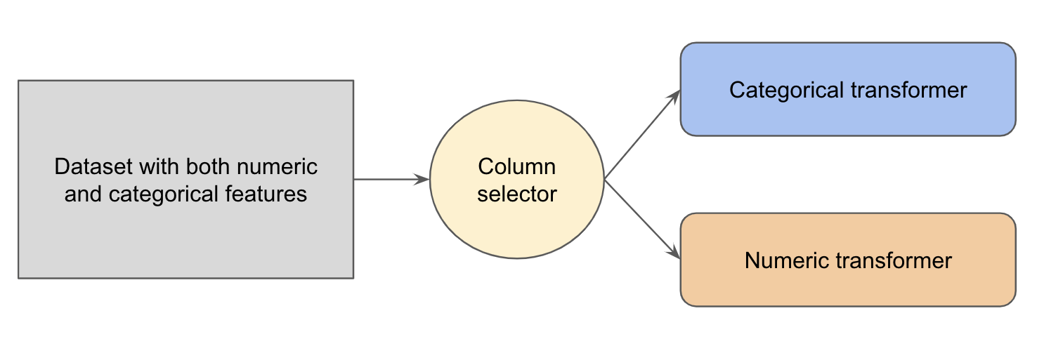
For a real life dataset we may have both numeric features and categorical features. It would be nice to selectively apply numeric transformation on the numeric features and categorical transformation on the categorical features. We can accomplish this goal by composing a ColumnTransformer.

The example below has columns with numeric values ('n1', 'n2', 'n3') and categorical values ('c1', 'c2').
data = {'n1': [20, 300, 400, None, 100],
      'n2': [0.1, None, 0.5, 0.6, None],
      'n3': [-20, -10, 0, -30, None],
      'c1': ['Male', 'Female', None, 'Female', 'Female'],
      'c2': ['Apple', 'Orange', 'Apple', 'Banana', 'Pear'],
    }

df = pd.DataFrame(data)

df
| n1 | n2 | n3 | c1 | c2 | |
|---|---|---|---|---|---|
| 0 | 20.0 | 0.1 | -20.0 | Male | Apple |
| 1 | 300.0 | NaN | -10.0 | Female | Orange |
| 2 | 400.0 | 0.5 | 0.0 | None | Apple |
| 3 | NaN | 0.6 | -30.0 | Female | Banana |
| 4 | 100.0 | NaN | NaN | Female | Pear |
A ColumnTransformer stores a list of (name, transformer, columns) tuples as transformers, which allows different columns to be transformed separately.
from sklearn.compose import ColumnTransformer

preprocessor = ColumnTransformer(
            transformers=[
                ("num", numeric_transformer, ["n1", "n2", "n3"]),
                ("cat", categorical_transformer, ["c1", "c2"]),
            ]
        )
We fit all transformers on dataset df, transform dataset df, and concatenate the results with method fit_transform.
preprocessor.fit_transform(df)
array([[-1.35411306, -1.95003374, -0.5       ,  0.        ,  1.        ,
         0.        ,  1.        ,  0.        ,  0.        ,  0.        ],
       [ 0.70649377,  0.3441236 ,  0.5       ,  1.        ,  0.        ,
         0.        ,  0.        ,  0.        ,  1.        ,  0.        ],
       [ 1.44242478,  0.3441236 ,  1.5       ,  0.        ,  0.        ,
         1.        ,  1.        ,  0.        ,  0.        ,  0.        ],
       [-0.02943724,  0.91766294, -1.5       ,  1.        ,  0.        ,
         0.        ,  0.        ,  1.        ,  0.        ,  0.        ],
       [-0.76536825,  0.3441236 ,  0.        ,  1.        ,  0.        ,
         0.        ,  0.        ,  0.        ,  0.        ,  1.        ]])
After fitting the transformers, we can use preprocessor on new dataset.
data_new = {'n1': [10],
      'n2': [None],
      'n3': [-10],
      'c1': ['Male'],
      'c2': [None],
    }

df_new = pd.DataFrame(data_new)
df_new
| n1 | n2 | n3 | c1 | c2 | |
|---|---|---|---|---|---|
| 0 | 10 | None | -10 | Male | None |
preprocessor.transform(df_new)
array([[-1.42770616,  0.3441236 ,  0.5       ,  0.        ,  1.        ,
         0.        ,  0.        ,  0.        ,  0.        ,  0.        ]])
Design Your Own Transformers
We can design custom transformers by defining a subclass of BaseEstimator and TransformerMixin. There are three methods we need to implement: __init__ , fit, and transform.
In the example below, we design a simple transformer to first fill missing values with zeros and divide the values by 10.
from sklearn.base import BaseEstimator, TransformerMixin


class CustomTransformer(BaseEstimator, TransformerMixin):

    def __init__(self) -> None:
        pass

    def fit(self, X: pd.DataFrame, y=None):
        return self

    def transform(self, X: pd.DataFrame, y=None):
        X = X.fillna(0)
        return X/10
Once the custom transformer is initialized, it can be used the same way as any other transformers we discussed before. Here we use the custom transformer on column "n3".
custom_tansformer = CustomTransformer()
preprocessor_custom = ColumnTransformer(
            transformers=[
                ("num", numeric_transformer, ["n1", "n2"]),
                ("custom", custom_tansformer, ["n3"]),
                ("cat", categorical_transformer, ["c1", "c2"]),
            ]
        )
preprocessor_custom.fit_transform(df)
array([[-1.35411306, -1.95003374, -2.        ,  0.        ,  1.        ,
         0.        ,  1.        ,  0.        ,  0.        ,  0.        ],
       [ 0.70649377,  0.3441236 , -1.        ,  1.        ,  0.        ,
         0.        ,  0.        ,  0.        ,  1.        ,  0.        ],
       [ 1.44242478,  0.3441236 ,  0.        ,  0.        ,  0.        ,
         1.        ,  1.        ,  0.        ,  0.        ,  0.        ],
       [-0.02943724,  0.91766294, -3.        ,  1.        ,  0.        ,
         0.        ,  0.        ,  1.        ,  0.        ,  0.        ],
       [-0.76536825,  0.3441236 ,  0.        ,  1.        ,  0.        ,
         0.        ,  0.        ,  0.        ,  0.        ,  1.        ]])
Conclusion
In summary, we discussed how data transformation can be constructed as a pipeline. We can fit a data transformation pipeline on our training dataset and use the same pipeline to transform new dataset.